Maze Generation Notes
I think I need to note that following has not been peer reviewed in anyway shape or form so is liable to contain egregious errors. For instance in the first couple paragraphs I realize that I'm solving a problem which probably does not need solving. Still I think my results for this work, though in search of a problem to solve are interesting.
Additionally I recently read "Maximal-entropy random walks in complex networks with limited information" by Roberta Sinatra, Et al. First I should have read this for my thesis. The biased random walks I used are in some cases equivalent to the maximal entropy random walks (MERW) in this paper and the walks in this paper are more formally justified than in my work. Unfortunately like many physics papers this it lacks some details like all graph sizes and in my experience some of the approximations described in the paper start to break down in graphs of tens or hundreds of thousands of nodes. Second I am unsure exactly how much the ideas formulated below differ from a MERW if at all. I may have simply designed an algorithm for generating an MERW transition matrix or I may not have. I'm simply not currently sure. This is a note to my future self to look into this and run some simulations (Dec. 2020).I needed to generate mazes for a project. I wanted to generate mazes of size $n$ ranging from $n=10$ to about $n=100$. Simple problem right, get a grid and start dropping walls. Wrong! It turns out that a maze where every location is accessible and there are no loops is equivalent to a spanning tree. A spanning tree is a path which visits every node in a graph exactly once without any cycles. Spanning trees appear some path finding algorithms but are interesting mathematical objects in their own right.
Although I have a background in graph theory, spanning trees were not my first thought when it came to maze generation, instead I thought of a random walk, a simple random walk to be specific. In a simple random walk given the walks current location you move with equal probability to every adjacent space or node, and the process repeats possibly forever.
So say $n=5$ meaning our maze is a grid with $5$ spaces on each side and $25$ spaces in total. Also lets define the maze entrance to be at space $(0,0)$ and exit to be at $(4,4)$. This gives the grid below.
If the simple random walk is at space $(0,0)$ and diagonal moves are not allowed then it has $\frac{1}{2}$ probability of moving to space $(0,1)$ and $\frac{1}{2}$ probability of moving to space $(1,0)$. If the random walk is allowed to backtrack, i.e. if the random walk is at space $(0,1)$ it is allowed to return to space $(0,0)$ then the random walk will continue indefinitely eventually visiting every space. Therefore if the random walk starts in location $(0,0)$ and we terminate it when it reaches space $(4,4)$ we have a random path from space $(0,0)$ to $(4,4)$.
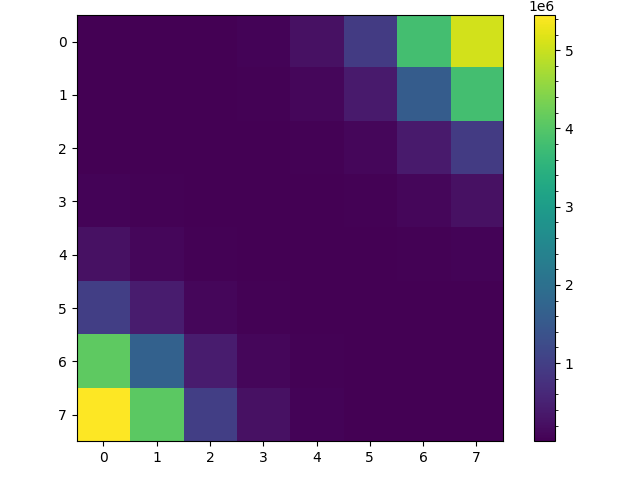
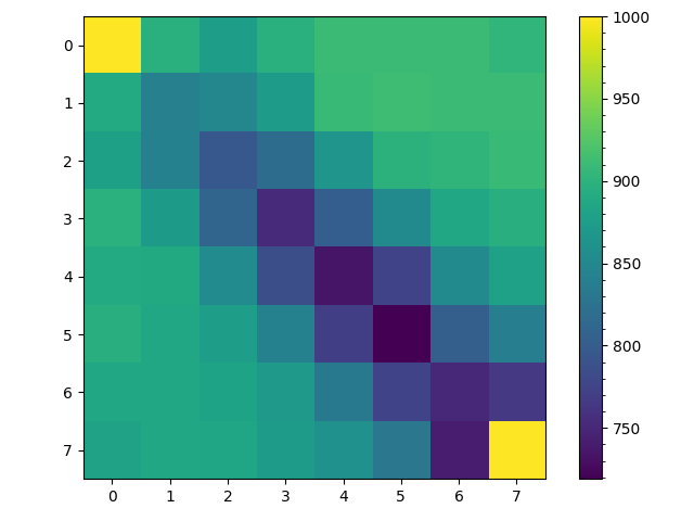
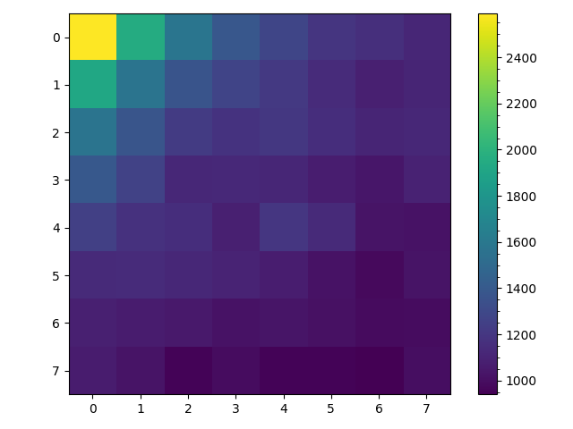
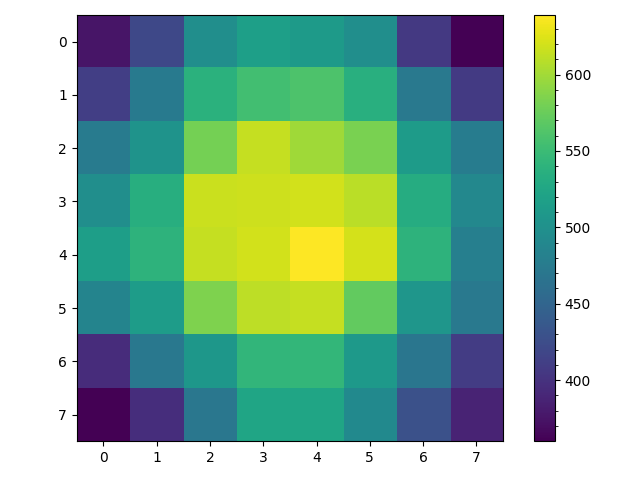
Of course this path may have loops and may either visit every space in our grid or only $9$ of the $25$ spaces. These are all potential problems with our generated maze but there is a more subtle problem. To see this ask assuming the random walk starts at $(0,0)$ and is not allowed to backtrack, what is the probability that on the second move the random walk arrives are space $(0,2)$? If the random walk arrives at space $(0,2)$ on the second move it had to be at space $(0,1)$ after the first move. So given that the probability of moving to space $(0,1)$ on the first move is $\frac{1}{2}$ and the given the random walk is at $(0,1)$ the probability of it moving to location $(0,2)$ is also $\frac{1}{2}$, the probability of arriving at space $(0,2)$ on the second move can be computed as follows, \begin{align} P((0,1)|(0,0)) &= \frac{1}{2}\\ P((0,2)|(0,1)) &= \frac{1}{2}\\ P((0,2)|(0,0)) &= P((0,1)|(0,0)) P((0,2)|(0,1)\\ &= \frac{1}{4} \end{align} Now ask what is the probability of arriving at space $(1,1)$ on the second move? Well its \begin{align} P((1,1)|(0,0)) &= P((0,1)|(0,0)) P((1,1)|(0,1) + P((1,0)|(0,0)) P((1,1)|(1,0)\\ &= \frac{1}{4} + \frac{1}{4}\\ &= \frac{1}{2} \end{align} In other words, the random walk is more likely to visit spaces along the diagonal then spaces along the edge of the grid. This is shown numerically in the two heatmaps below. These are generated from $1000$ random walks starting at $(0,0)$ and ending at $(7,7)$. The figure on the left counts all visits to a space and we see that the random walks spend most of their time near where they begin at space $(0,0)$. But since we are uninterested in repeated visits to a space in maze generation the right is more useful, it counts each time a space was visited at least once in each of the $1000$ random walks from $(0,0)$ to $(7,7)$. Here it is clear that nearly all random walks pass through the spaces along the diagonal from space $(0,0)$ to $(7,7)$ but only about half make it to spaces $(0,7)$ and $(7,0)$.
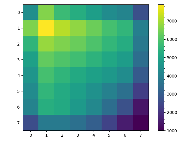
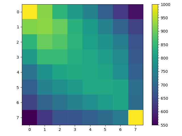
This is perhaps less of a problem then I initially thought. If we look at the left figure excluding the edges the probability of being in any space along a counter diagonal (diagonal right to left) is actually pretty uniform with the number of visits to a space being more of a function of distance from the end location $(7,7)$ then anything else. Also while only about half the random walks visit space $(0,7)$ and $(7,0)$ on a given walk, a random walk by definition does not necessarily visit every state or space.
So if your really only interested in maze generation a naive random walk will probably work just fine. But could we do better or at least change the characteristics of the random walk to change the texture of the resulting mazes which from the right figure would appear to be solvable by simply traversing the diagonal? I don't know, I mean how do we define "better" or the "texture" of a maze. But perhaps we can at least change the characteristics of the random walk which generates the maze.
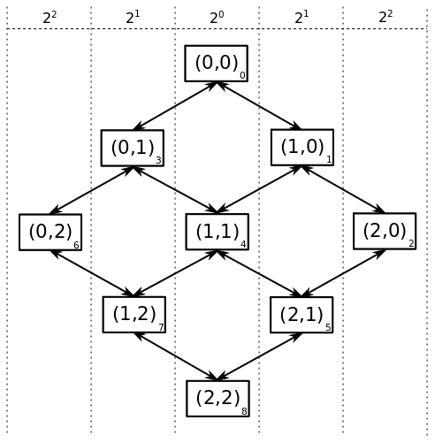
To increase the chance of the random walk reaching the edges of the gird instead of using a simple random walk which moves to all adjacent squares with equal probability, I decided adjust the transition probabilities so that the random walk is more likely to visit edge spaces such as $(0,7)$ and $(7,0)$. If it is possible to find an exact solution to this problem such that the probability of visiting any square on the counter diagonal is equal using Markov chain theory I would really like to know how! Below I will go into two approaches I took to try finding an "exact" solution the second of which was more successful then the first. But generally being lazy, instead of pursuing an exact solution I first choose to try a rough approximation. The basic problem we observed above is that if we approximate the undirected graph the simple random walk traverses as a directed graph, the probability of visiting space $(1,1)$ at $m=2$ is twice that of visiting space $(0,2)$. The following figures show the true undirected graph on the left and my approximation of it with a directed graph on the right for $n=3$.
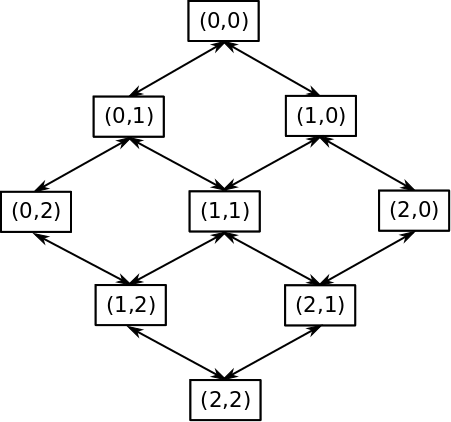
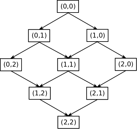
I decided to try a random walk biasing scheme that should push the random walk toward the edges of the maze. The figure below gives the bias scheme, bias $2^0=1$ for the diagonal nodes $(0,0)$, $(1,1)$, and $(2,2)$, bias of $2^1=2$ for $1$ step left and right of the diagonal, and generally $2^x$ for $x$ steps off the diagonal. More generally letting the tuple indexing each node be represented as $(i,j)$ we can compute $x$ as $x=abs(i-j)$ and therefore the bias at node $(i,j)$ is $b_{i,j}=2^{abs(i-j)}$.
 These biases can be put into a transition matrix and then row normalized so the probability of leaving any space is $1$. In the transition matrix below $n=3$ and row and column labels correspond to the numbers in the lower left corners of the biasing figure above.
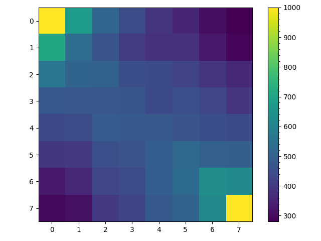
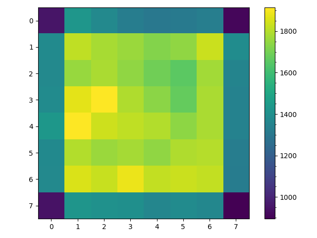
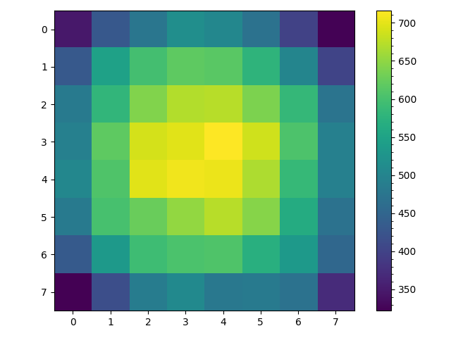
Running a random walk $1000$ times using this biasing scheme with a grid of size $n=8$ gives the following heatmaps. The one on the left counts all visits to a space and the one on the right just the first visit. In both its clear that the edge spaces are visited more often then in the case of the unbiased random walk, in fact the diagonal spaces are now less visited than the edge spaces.
Adding some additional ad-hoc techniques to fill out the maze with branches from solution path generated using the biased random walk technique described above gives an algorithm that can produce an arbitrarily sized maze such as the one shown below.
Notions of Uniformity in Maze Generation
In the following section I distinguish between the notion of uniformity used by Wilson in his algorithm for constructing spanning trees described in "Generating Random Spanning Trees More Quickly than the Cover Time" and the notion I use above. The brief explanation is that Wilson's notion of uniformity gives guarantees on the probability of a given spanning tree being selected from the set of possible spanning trees. As a maze without any loops or disconnected spaces is equivalent to a spanning tree, Wilson's algorithm gives guarantees on the probability of the generating a given maze using his algorithm. On the other hand the biased random walk algorithms above attempt to achieve an uniformity in the sense that the mazes solution path has equal probability of visiting each space in the counter diagonal of the maze; where this probability is less than one and the maze starts in the upper left corner and ends in the lower right. None of my algorithms achieve my notion of uniformity but I think they represent a step or two in that direction.
Wilson's Notion:
Wilson defines that weight of a spanning tree as follows "The weight of a spanning tree, with edges directed towards its root is the product of the weight of its edges". Since I am unconcerned here with directed graphs lets simplify Wilson's definition to simply the product of the weights of the trees edges. This definition is different from the more common definition of the weight of a spanning tree as the sum of the trees edge weights used in the definition of a minimum spanning tree (MST).
Regardless, Wilson uses this definition of a spanning tree weight to define $\mathscr{Y}_r(G)$ as the probability distribution given graph $G$ of constructing a spanning tree rooted at node $r$ such that the probability of constructing a spanning tree is proportional to its weight. Whether heavy spanning trees are more or less likely in $\mathscr{Y}_r(G)$ is unclear. What is clear is that all the trees of equal weight have equal probability of being constructed under distribution $\mathscr{Y}_r(G)$. Therefore if on an $(n\times n)$ grid the weights of all possible paths between adjacent spaces in a maze are equal, all the spanning trees representing these possible mazes have equal weight, and all of these spanning trees are generated with the same probability. In this sense, Wilson's algorithm can be said to sample uniformly from the set of possible mazes on an $(n\times n)$ grid.
My Notion:
I defined my notion of uniformity in regards to a related by fundamentally different problem. The problem is related in so far as Wilson's algorithm constructs a maze and I initially thought my attempts to generate a random path solving the maze were equivalent problems. They are not.
Yet knowing that Wilson's algorithm selected uniformly from the set of mazes, I initially thought the algorithm also selected uniformly from the set of paths solving the maze. However it is not clear that it does. In fact my notion of constructing a random path solving the maze such that all spaces on the counter diagonal of a grid have equal probability of being visited is both fundamentally different then Wilson's notion of uniformity and is poorly defined.
Lets take a stab at making my notion of uniformity in random path generation more rigorous. Given an $(n\times n)$ grid $G$ where $G(r,c)$ is the space in the $r_{th}$ row and $c_{th}$ column of $G$, $G(1,1)$ is the upper left space, and $G(n,n)$ the lower right. Define adjacency on the grid for space $G(r,c)$ as $G \bigcap \{G(r+1,c),G(r-1,c),G(r,c+1),G(r,c-1)\}$ the set of spaces vertically and horizontally adjacent to $G(r,c)$. Further define the set of spaces \begin{equation} \mathcal{D}_i := \{G(r,c)|r+c = i+1, 1\leq r \leq n, 1\leq c \leq n\} \end{equation} as the $i_{th}$ counter diagonal.
This allows us to define the sets of equal probability spaces as \begin{equation} \mathcal{W}_j := \{G(r,c) | G(r,c)\in\mathcal{D}_i, |\mathcal{D}_i|=j, 1\leq j \leq n\} \end{equation} Now let k-tuple $\mathbf{r}$ be a path in $G$ consisting of adjacent spaces and define the following set \begin{equation} \mathcal{U} := \{\mathbf{r} | i\neq j \iff \mathbf{r}(i) \neq \mathbf{r}(j), 1\leq i\leq k, 1\leq j\leq k \} \end{equation} as the paths in $G$ without cycles. This set of non-cyclic paths can be reduced to the set of paths which start at $G(1,1)$ and end at $G(n,n)$ as \begin{equation} \mathcal{R} := \{\mathbf{r} | \mathbf{r}(1)=G(1,1), \mathbf{r}(k)=G(n,n), \mathbf{r} \in \mathcal{U}\} \end{equation}
Given an algorithm $A(G)$ for generating a random path on $G$. Let $A(G)$ generate a valid collection $\mathfrak{R}$ of $q$ paths. Where validity is defined as \begin{equation} \mathbf{r} \in \mathfrak{R} \implies \mathbf{r} \in \mathcal{R} \end{equation} and using the set of paths $\mathfrak{R}$ generated with $A(G)$ let, \begin{equation} y_{r,c} = \sum_{\mathbf{r} \in \mathfrak{R}, G(x,y)\in\mathbf{r}} \mathbb{1}_{\bigg((x,y)=(r,c)\bigg)} \end{equation} where $\mathbb{1}_{(\ast)}$ is the indicator function. $y_{r,c}$ is the count of the number of times space $G(r,c)$ is visited by the paths in set $\mathfrak{R}$.
Finally we can define my notion of random path generation as being uniform in the number of times paths in set $\mathfrak{R}$ visit spaces in set $\mathcal{W}_j$ of equal probable spaces along counter diagonals of length $j$ as being satisfied if for any $j$ and any $y_{r,c}\in\mathcal{W}_j$ and $y_{x,y}\in\mathcal{W}_j$, \begin{equation} y_{r,c} \approx y_{x,y} \end{equation} or more formally for arbitrary number $\epsilon > 0$, \begin{equation} \lim_{q\to\infty} Pr(|y_{r,c}-y_{x,y}| > \epsilon) =0 \end{equation} in other words algorithm $A(G)$ is uniform in the probability of its paths visiting a space in $G$'s counter diagonals if $y_{r,c}$ and $y_{x,y}$ converge in probability.
Now as defined above $\mathfrak{R}$ does not necessarily cover all elements of $\mathcal{R}$. For this to be the case algorithm $A(G)$ must generate a valid collection $\mathfrak{R}'$ of $q$ paths. Where validity is defined as \begin{equation} \mathbf{r} \in \mathfrak{R} \iff \mathbf{r} \in \mathcal{R} \end{equation} Substituting $\mathfrak{R}'$ for $\mathfrak{R}$ above the rest of the argument is exactly the same as above.
Sources:
$^{(1)}$ https://en.wikipedia.org/wiki/Spanning_tree
$^{(2)}$ https://en.wikipedia.org/wiki/Maze_generation_algorithm
$^{(3)}$ http://www.astrolog.org/labyrnth/algrithm.htm
$^{(4)}$ "Generating Random Spanning Trees More Quickly than the Cover Time" by David Wilson
An Exact Solution?
I mentioned that I had tried to find an exact solution for a biased transition matrix given a desired probability distribution of visiting each space in the grid. Well I'm not sure I have a general solution but I might have a specific one, which at least generates nice figures!
Say $n=3$, we have $9$ states, and we assume that the random walk starts at state $0$. Now lets look at how the probability of a simple random walk (left) vs my target probability (right) being in a given state changes with each step of the random walk.
$step=0$
$step=1$
$step=2$
$step=3$
$step=4$
Take away, first the probability of being in any given state under a simple random walk is not the same my target probability after step $2$. Second, notice that step $4$ of our target probability distribution has achieved "saturation" having reached all squares of the grid and simply oscillates between the distribution in step $3$ and $4$ for every step that follows.
Attempt 1
I first tried to take a linear algebra approach to finding the transition matrices which would achieve my target distributions at each step. Lets define the grid state at $step=0$ as a vector $v_0$, the grid state at $step=1$ as $v_1$, and the grid state at $step=i$ as $v_i$. Each vector $v_i$ is straightforward to compute given $v_0$. The question is how to compute a transition matrix $T_{0,1}$ given vectors $v_0$ and $v_1$? This is simple to express, \begin{align} v_0 T_{0,1} &= v_1\\ T_{0,1} &= v_0^{-1}v_1 \end{align} Unfortunately the inverse of $v_0$ does not exist since it is not a square matrix. But since $v_0$ is a row matrix consisting of a single column it follows that its columns are linearly independent. Therefore $$ v_0^+v_0 = I $$ where $v_0^+$ is the Moore-Penrose inverse or pseudo-inverse and $I$ is the identity matrix. Therefore if $v_0^+$ is computable then \begin{align} v_0 T_{0,1} &= v_1\\ v_0^+ v_0 T_{0,1} &= v_0^{+}v_1\\ I T_{0,1} &= v_0^{+}v_1\\ T_{0,1} &= v_0^{+}v_1\\ \end{align} One can compute the Moore-Penrose inverse $v_0^+$ as \begin{equation} v_0^+ = v_0^T\left(v_0v_0^T\right)^{-1} \end{equation} Unfortunately since $v_{0}$ is at least half zeros it follows that $v_{0}v_{0}^T$ is singular and its inverse $\left(v_{0}v_{0}^T\right)^{-1}$ does not exist. However in the limit \begin{equation} v_{0}^+ = \lim_{\delta \to 0} \left( A^*A + \delta I \right)^{-1} A^* = \lim_{\delta \to 0} A^* \left( A^*A + \delta I \right)^{-1} \end{equation} which is the Tikonov Regularization. Where $A^*$ is the Hermitian transpose which reduced to a simple transpose of $A$ if it is real matrix and $\delta$ is an arbitrarily small number. So subbing in $v_0$ for $A$ gives \begin{equation} v_{0}^+ = \lim_{\delta \to 0} \left( v_0^Tv_0 + \delta I \right)^{-1} v_0^T \end{equation}
Given $v_0$ we can compute $v_1,v_2,\ldots,v_i$ and therefore have \begin{align} v_0^{+}v_1 &= T_{0,1}\\ v_1^{+}v_2 &= T_{1,2}\\ \ldots\\ v_{i-1}^{+}v_i &= T_{i-1,i} \end{align} Lastly I row normalize to $1$ the rows of the resulting transition matrices $T_{i-1,i}$.
Unfortunately this approach does not work, but not in they way I expected like $v_0T_{0,1}\neq v_1$. Lets take for example $i=4$ and we know \begin{align} v_3 &= \left[0,\frac{1}{4},0,\frac{1}{4},0,\frac{1}{4},0,\frac{1}{4},0\right]\\ v_4 &= \left[\frac{1}{5},0,\frac{1}{5},0,\frac{1}{5},0,\frac{1}{5},0,\frac{1}{5}\right]\\ \end{align} Now the algorithm above gives, \begin{align} T_{3,4} &= \left[ \begin{array}{ccccccccc} 0 &0 &0 &0 &0 &0 &0 &0 &0\\ \frac{1}{5} &0 &\frac{1}{5} &0 &\frac{1}{5} &0 &\frac{1}{5} &0 &\frac{1}{5}\\ 0 &0 &0 &0 &0 &0 &0 &0 &0\\ \frac{1}{5} &0 &\frac{1}{5} &0 &\frac{1}{5} &0 &\frac{1}{5} &0 &\frac{1}{5}\\ 0 &0 &0 &0 &0 &0 &0 &0 &0\\ \frac{1}{5} &0 &\frac{1}{5} &0 &\frac{1}{5} &0 &\frac{1}{5} &0 &\frac{1}{5}\\ 0 &0 &0 &0 &0 &0 &0 &0 &0\\ \frac{1}{5} &0 &\frac{1}{5} &0 &\frac{1}{5} &0 &\frac{1}{5} &0 &\frac{1}{5}\\ 0 &0 &0 &0 &0 &0 &0 &0 &0\\ \end{array} \right] \end{align} Clearly its true that, \begin{equation} v_3 T_{3,4} = v_4 \end{equation} However recall the grid the random walk is traversing,
Attempt 2
I'm going to be a bit handwavy about this solution because I have not formalized it or tried to prove that it is correct. Its an algorithmic solution which given subsequent probability distributions of the possible locations on the random walk at time $v_i$ and $v_{i+1}$ computes the transition matrix T_{i,i+1}. For example lets take $i=3$ for $n=3$ such that, \begin{align} v_3 &= \left[0,\frac{1}{4},0,\frac{1}{4},0,\frac{1}{4},0,\frac{1}{4},0\right]\\ v_4 &= \left[\frac{1}{5},0,\frac{1}{5},0,\frac{1}{5},0,\frac{1}{5},0,\frac{1}{5}\right]\\ \end{align}
This implies that at time $i=3$ the random walk could be at the following locations $l_3=[1,3,5,7]$ and could transition to locations $l_4=[0,2,4,6,8]$. But given the restriction that the random walk only move one space along a vertical for horizontal access only the following transitions are possible. \begin{align} 1 \to [0,2,4]\\ 3 \to [0,4,6]\\ 5 \to [2,4,8]\\ 7 \to [4,6,8]\\ \end{align}
Marking these transitions in a transition matrix with $-1$ gives, \begin{align} T_{3,4} &= \left[ \begin{array}{ccccccccc} 0 &0 &0 &0 &0 &0 &0 &0 &0\\ -1 &0 &-1 &0 &-1 &0 &0 &0 &0\\ 0 &0 &0 &0 &0 &0 &0 &0 &0\\ -1 &0 &0 &0 &-1 &0 &-1 &0 &0\\ 0 &0 &0 &0 &0 &0 &0 &0 &0\\ 0 &0 &-1 &0 &-1 &0 &0 &0 &-1\\ 0 &0 &0 &0 &0 &0 &0 &0 &0\\ 0 &0 &0 &0 &-1 &0 &-1 &0 &-1\\ 0 &0 &0 &0 &0 &0 &0 &0 &0\\ \end{array} \right] \end{align}
Now first as a transition matrix after the transition values are filled in every row sum with non-zero elements should equal $1$ and every column sum should be \begin{equation} col\_sum_{i,i+1} = \frac{p_{i+1}}{p_i} \end{equation} where $p_i$ is the non-zero probability of being at a location at iteration $i$. So for $i=3$, \begin{equation} col\_sum_{3,4} = \frac{\frac{1}{5}}{\frac{1}{4}} = \frac{4}{5} \end{equation}
The algorithm then selects the column or row with preference for the columns with the fewest unset elements. If the current probability sum of a column is $col\_sum'=\frac{1}{2}$ and there are two unset elements, assign each element probability $\frac{1}{4}$. If assigning probability $\frac{1}{4}$ to one of these elements would violate a row sum assign that element probability $p'$such that the row sum equals $1$ and the rest of the probability $p'' = col\_sum - (col\_sum' + p')$ to the second element. The same basic procedure is followed in setting the transition probabilities in a row of the transition matrix.
For example filling in the columns with two unset elements gives \begin{align} T_{3,4} &= \left[ \begin{array}{ccccccccc} 0 &0 &0 &0 &0 &0 &0 &0 &0\\ \frac{2}{5} &0 &\frac{2}{5} &0 &-1 &0 &0 &0 &0\\ 0 &0 &0 &0 &0 &0 &0 &0 &0\\ \frac{2}{5} &0 &0 &0 &-1 &0 &\frac{2}{5} &0 &0\\ 0 &0 &0 &0 &0 &0 &0 &0 &0\\ 0 &0 &\frac{2}{5} &0 &-1 &0 &0 &0 &\frac{2}{5}\\ 0 &0 &0 &0 &0 &0 &0 &0 &0\\ 0 &0 &0 &0 &-1 &0 &\frac{2}{5} &0 &\frac{2}{5}\\ 0 &0 &0 &0 &0 &0 &0 &0 &0\\ \end{array} \right] \end{align} This forces the rest of the unset values to be $\frac{1}{5}$ giving, \begin{align} T_{3,4} &= \left[ \begin{array}{ccccccccc} 0 &0 &0 &0 &0 &0 &0 &0 &0\\ \frac{2}{5} &0 &\frac{2}{5} &0 &\frac{1}{5} &0 &0 &0 &0\\ 0 &0 &0 &0 &0 &0 &0 &0 &0\\ \frac{2}{5} &0 &0 &0 &\frac{1}{5} &0 &\frac{2}{5} &0 &0\\ 0 &0 &0 &0 &0 &0 &0 &0 &0\\ 0 &0 &\frac{2}{5} &0 &\frac{1}{5} &0 &0 &0 &\frac{2}{5}\\ 0 &0 &0 &0 &0 &0 &0 &0 &0\\ 0 &0 &0 &0 &\frac{1}{5} &0 &\frac{2}{5} &0 &\frac{2}{5}\\ 0 &0 &0 &0 &0 &0 &0 &0 &0\\ \end{array} \right] \end{align} Notice that all rows sum to $1$ and all columns sum to $\frac{4}{5}$.This is a particularly easy transition matrix to compute and in fact filling out these transition matrices by hand for small $n$ is generally pretty straightforward. Formalizing and proving the correctness of an algorithm for arbitrary $n$ is much more difficult. This algorithm also solves an undetermined problem, so the transition matrices produced by this algorithm are not necessarily unique.
The Conditioned Backtracking Algorithm
The algorithm above allows us to compute a conditioned transition matrix, conditioned on $v_i$ and $v_{i+1}$ the algorithm produces $T_{i,i+1}$. However this algorithm also conditions on the starting position $0$ and ending position $8$ of the random walk. So for $n=3$ as we saw above this gives the following location vectors and transition matrices.
\begin{align} \begin{array}{c} v_0\\ --\\ 1\\ 0\\ 0\\ 0\\ 0\\ 0\\ 0\\ 0\\ 0\\ \end{array} \to T_{0,1} \to \begin{array}{c} v_1\\ --\\ 0\\ \frac{1}{2}\\ 0\\ \frac{1}{2}\\ 0\\ 0\\ 0\\ 0\\ 0\\ \end{array} \to T_{1,2} \to \begin{array}{c} v_2\\ --\\ \frac{1}{4}\\ 0\\ \frac{1}{4}\\ 0\\ \frac{1}{4}\\ 0\\ \frac{1}{4}\\ 0\\ 0\\ \end{array} \to T_{2,3} \to \begin{array}{c} v_3\\ --\\ 0\\ \frac{1}{4}\\ 0\\ \frac{1}{4}\\ 0\\ \frac{1}{4}\\ 0\\ \frac{1}{4}\\ 0\\ \end{array} \to T_{3,4} \to \begin{array}{c} v_4\\ --\\ \frac{1}{5}\\ 0\\ \frac{1}{5}\\ 0\\ \frac{1}{5}\\ 0\\ \frac{1}{5}\\ 0\\ \frac{1}{5}\\ \end{array} \to \text{(Stop if walk is at space $8$. Else...)} \to \begin{array}{c} v_2\\ --\\ \frac{1}{4}\\ 0\\ \frac{1}{4}\\ 0\\ \frac{1}{4}\\ 0\\ \frac{1}{4}\\ 0\\ 0\\ \end{array} \to T_{2,3} \to \ldots \end{align} Note that the looping back to $v_2$ is conditioned on it not having arrived at space $8$, if it had the random walk would have terminated. Therefore distribution $v_4$ collapses to $v_2$ and the algorithm loops.
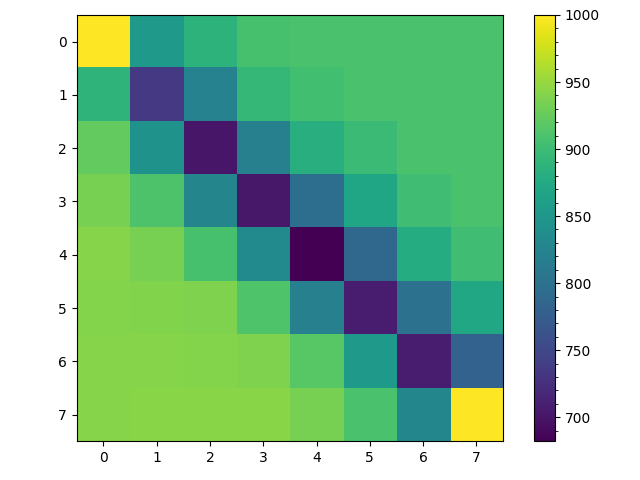
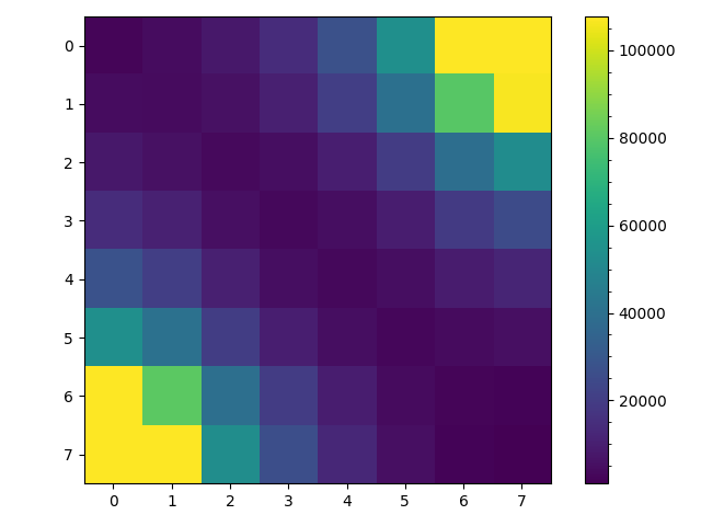
The result of this algorithm are given below. On the left is a heat map for the number of visits to each space given $1000$ trials. On the right is a heat map for the number of walks of the $1000$ trials that visited as space at least once.
The left figure demonstrates that in one sense we have achieved our goal. Counting all visits to a space is proportional to the steady state probability of being in a space and the counter diagonals are approximately uniform including for spaces along the edge. But given backtracking the steady state probability of actually being in any space is not actually fairly uniform as random walks near space $0$ tend to stay in that area while random walks near space $63$ tend to terminate over a given time period. Instead the steady state probability displays a gradient from the upper left to the lower right corner.
The right figure shows that the difference in the spaces visited at least once per walk using this algorithm is to very different from the simple random walk. The difference between the corner spaces $(0,7)$, $(7,0)$ and $(3,3)$, $(4,4)$ are between $200$ and $300$ walks, perhaps with more trials or for larger $n$ the difference would be greater. But one apparent difference is that the random walk using this transition matrix appears to pend less time wandering before reaching termination. Roughly speaking in the simple random walk the average space is visited $800$ out of $1000$ trials while in this biased random walk each space appears visited on average $600$ of the $1000$ trials.
Aside: I wonder if by shifting probability weight away from the spaces near $(0,0)$ and toward $(7,7)$ each iteration would reduce or eliminate the gradient in the count of all visits to a space? Naively, I don't see any reason why it wouldn't work.
The Conditioned Non-Backtracking Algorithm
But say we eliminated backtracking giving the following progression of possible distributions, \begin{align} \begin{array}{c} v_0\\ --\\ 1\\ 0\\ 0\\ 0\\ 0\\ 0\\ 0\\ 0\\ 0\\ \end{array} \to T_{0,1} \to \begin{array}{c} v_1\\ --\\ 0\\ \frac{1}{2}\\ 0\\ \frac{1}{2}\\ 0\\ 0\\ 0\\ 0\\ 0\\ \end{array} \to T_{1,2} \to \begin{array}{c} v_2\\ --\\ 0\\ 0\\ \frac{1}{3}\\ 0\\ \frac{1}{3}\\ 0\\ \frac{1}{3}\\ 0\\ 0\\ \end{array} \to T_{2,3} \to \begin{array}{c} v_3\\ --\\ 0\\ 0\\ 0\\ 0\\ 0\\ \frac{1}{2}\\ 0\\ \frac{1}{2}\\ 0\\ \end{array} \to T_{3,4} \to \begin{array}{c} v_4\\ --\\ 0\\ 0\\ 0\\ 0\\ 0\\ 0\\ 0\\ 0\\ 1\\ \end{array} \end{align} Would that produce a steady state distribution closer to initial goal of uniformly colored counter diagonals? The answer given in the figure below is yes, but unfortunately such a random walk will not produce a particularly interesting maze.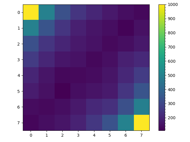
The Unconditioned Backtracking Algorithm
Finally lets test unconditioning on the starting location of the random walk and instead selecting them uniformly at random. This can be represented as the following location vectors $v_0$, $v_1$ and transition matrices $T_{0,1}$, $T_{1,0}$. \begin{align} \begin{array}{c} v_0\\ --\\ 0\\ \frac{1}{4}\\ 0\\ \frac{1}{4}\\ 0\\ \frac{1}{4}\\ 0\\ \frac{1}{4}\\ 0\\ \end{array} \to T_{0,1} \to \begin{array}{c} v_1\\ --\\ \frac{1}{5}\\ 0\\ \frac{1}{5}\\ 0\\ \frac{1}{5}\\ 0\\ \frac{1}{5}\\ 0\\ \frac{1}{5}\\ \end{array} \to T_{1,0} \to \begin{array}{c} v_0\\ --\\ 0\\ \frac{1}{4}\\ 0\\ \frac{1}{4}\\ 0\\ \frac{1}{4}\\ 0\\ \frac{1}{4}\\ 0\\ \end{array} \to\ldots \end{align} Interestingly if $r_1(X)$ is a function which row normalizes the rows of matrix $X$ and $X^{'}$ is the transpose of matrix $X$ then, \begin{equation} T_{1,0} = r_1(T_{0,1}^{'}) \end{equation} Additionally since the non-zero rows and columns of $T_{0,1}$ and independent of those of $T_{1,0}$ these two matrices can be combined into one stochastic matrix $T$, \begin{equation} T = T_{0,1} + T_{1,0} \end{equation} Selecting a starting space uniformly at random and running $1000$ random walks for $100$ steps each produced the following figures. The left figure counts all visits to a space and noticing that the color scale has a range of about $250$ is fairly uniform relative to the other figures. The right figure counts only the first time a random walk visits a space. We see that most walks visit the center spaces and less then half the walks visit the corner spaces.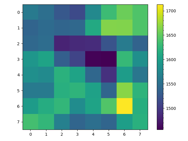
So in conclusion, can any of this work be adapted to solve problems in the real world? Well at the moment I'm not sure.